
Apparently, you can teach an old dog new tricks.
Last year I wrote a blog post about building a data processing pipeline using DuckDB to ingest weather sensor data from the UK’s Environment Agency. The pipeline was based around a set of SQL scripts, and whilst it used important data engineering practices like data modelling, it sidestepped the elephant in the room for code-based pipelines: dbt.
dbt (data build tool) is an open-source tool that lets data engineers write the transformation layer of a data pipeline as modular SQL (with some Jinja templating on top), and brings with it all the good stuff you’d expect from a mature tool: testing, documentation, dependency management, incremental loads, and more. Created in 2016, it really exploded in popularity on the data engineering scene around 2020. This also coincided with my own journey away from hands-on data engineering and into Kafka and developer advocacy. As a result, dbt has always been one of those things I kept hearing about but never tried.
I’m rather delighted to say that as of today, dbt has definitely 'clicked'. How do I know? Because not only can I explain what I’ve built, but I’ve even had the 💡 lightbulb-above-the-head moment seeing it in action and how elegant the code used to build pipelines with dbt can be.
In this blog post I’m going to show off what I built with dbt, contrasting it to my previous hand-built method.
| You can find the full dbt project on GitHub here, and read about how I had Claude teach me dbt. |
If you’re new to dbt hopefully it’ll be interesting and useful. If you’re an old hand at dbt then you can let me know any glaring mistakes I’ve made :)
First, a little sneak peek:

Now, let’s look at how I did it.
The Data 🔗
| I’m just going to copy and paste this from my previous article :) |
At the heart of the data are readings, providing information about measures such as rainfall and river levels. These are reported from a variety of stations around the UK.

The data is available on a public REST API (try it out here to see the current river level at one of the stations in Sheffield).
|
I’ve used this same set of environment sensor data many times before, because it provides just the right balance of real-world imperfections, interesting stories to discover, data modelling potential, and enough volume to be useful but not too much to overwhelm. |
Ingest 🔗
What better place to start from than the beginning?
Whilst DuckDB has built-in ingest capabilities (which is COOL) it’s not necessarily the best idea to tightly couple ingest with transformation.
Previously I did it one-shot like this:
CREATE OR REPLACE TABLE readings_stg AS
  WITH src AS (
    SELECT * (1)
      FROM read_json('https://environment.data.gov.uk/flood-monitoring/data/readings?latest')) (1)
    SELECT u.* FROM (
SELECT UNNEST(items) AS u FROM src); (2)| 1 | Extract |
| 2 | Transform |
dbt encourages a bit more rigour with the concept of sources. By defining a source we can decouple the transformation of the data (2) from its initial extraction (1). We can also tell dbt to use a different instance of the source (for example, a static dataset if we’re on an aeroplane with no wifi to keep pulling the API), as well as configure freshness alerts for the data.
The staging/sources.yml defines the data source:
[…]
  - name: env_agency
    schema: main
    description: Raw data from the [Environment Agency flood monitoring API](https://environment.data.gov.uk/flood-monitoring/doc/reference)
    tables:
      - name: raw_stations
[…]
Note the description - this is a Markdown-capable field that gets fed into the documentation we’ll generate later on.
It’s pretty cool.
So env_agency is the logical name of the source, and raw_stations the particular table.
We reference these thus when loading the data into staging:
SELECT
    u.dateTime, u.measure, u.value
FROM (
    SELECT UNNEST(items) AS u
    FROM {{ source('env_agency', 'raw_readings') }} (1)
)| 1 | referencing the source |
So if we’re not pulling from the API here, where are we doing it?
This is where we remember exactly what dbt is—and isn’t—for. Whilst DuckDB can pull data from an API directly, it doesn’t map directly to capabilities in dbt for a good reason—dbt is for transforming data.
That said, dbt is nothing if not flexible, and its ability to run Jinja-based macros gives it superpowers for bending to most wills. Here’s how we’ll pull in the readings API data:
{% macro load_raw_readings() %}
{% set endpoint = var('api_base_url') ~ '/data/readings?latest' %} (1)

{% do log("raw_readings ~ reading from " ~ endpoint, info=true) %}

{% set sql %}
    CREATE OR REPLACE TABLE raw_readings AS
    SELECT *,
            list_max(list_transform(items, x -> x.dateTime)) (2)
            AS _latest_reading_at                            (2)
    FROM read_json('{{ endpoint }}') (3)
{% endset %}
{% do run_query(sql) %}

{% do log("raw_readings ~  loaded", info=true) %}

{% endmacro %}| 1 | Variables are defined in dbt_project.yml |
| 2 | Disassemble the REST payload to get the most recent timestamp of the data, store it as its own column for freshness tests later |
| 3 | As it happens, we are using DuckDB’s read_json to fetch the API data (contrary, much?) |
Even though we are using DuckDB for the extract phase of our pipeline, we’re learning how to separate concerns. In a 'real' pipeline we’d use a separate tool to load the data into DuckDB (I discuss this a bit further later on). We’d do it that way to give us more flexibility over things like retries, timeouts, and so on.
The other two tables are ingested in a similar way, except they use CURRENT_TIMESTAMP for _latest_reading_at since the measures and stations APIs don’t return any timestamp information.
If you step away from APIs and think about data from upstream transactional systems being fed into dbt, there’ll always be (or should always be) a field that shows when the data last changed.
Regardless of where it comes from, the purpose of the _latest_reading_at field is to give dbt a way to understand when the source data was last updated.
In the staging/sources.yml the metadata for the source can include a freshness configuration:
[…]
  - name: env_agency
    tables:
      - name: raw_stations
        loaded_at_field: _latest_reading_at
        freshness:
          warn_after: { count: 24, period: hour }
          error_after: { count: 48, period: hour }
[…]
This is the kind of thing where the light started to dawn on me that dbt is popular with data engineers for a good reason; all of the stuff that bites you in the ass on day 2, they’ve thought of and elegantly incorporated into the tool. Yes I could write yet another SQL query and bung it in my pipeline somewhere that checks for this kind of thing, but in reality if the data is stale do we even want to continue the pipeline?
With dbt we can configure different levels of freshness check—"hold up, this thing’s getting stale, just letting you know" (warning), and "woah, this data source is so old it stinks worse than a student’s dorm room, I ain’t touching either of those things" (error).
Thinking clearly 🔗
When I wrote my previous blog post I did my best to structure the processing logically, but still ended up mixing pre-processing/cleansing with logical transformations.
dbt’s approach to source / staging / marts helped a lot in terms of nailing this down and reasoning through what processing should go where.
For example, the readings data is touched three times, each with its own transformations:
-
Ingest: get the data in
CREATE OR REPLACE TABLE raw_readings AS
SELECT *, (1)
        list_max(list_transform(items, x -> x.dateTime)) (2)
        AS _latest_reading_at (2)
FROM read_json('{{ endpoint }}')
1 raw data, untransformed 2 add a field for the latest timestamp -
Staging: clean the data up
SELECT
    u.dateTime,
    {{ strip_api_url('u.measure', 'measures') }} AS measure, (1)
    CAST( (2)
        CASE WHEN json_type(u.value) = 'ARRAY' THEN u.value->>0 (2)
             ELSE CAST(u.value AS VARCHAR)(2)
        END AS DOUBLE(2)
    ) AS value(2)
FROM (
    SELECT UNNEST(items) AS u (3)
    FROM {{ source('env_agency', 'raw_readings') }}
)
1 Drop the URL prefix from the measure name to make it more usable 2 Handle situations where the API sends multiple values for a single reading (just take the first instance) 3 Explode the nested array Except for exploding the data, the operations are where we start applying our opinions to the data (how
measureis handled) and addressing data issues (valuesometimes being a JSON array with multiple values) -
Marts: build specific tables as needed, handle incremental loads, backfill from archive, etc
{{
    config(
        materialized='incremental',
        unique_key=['dateTime', 'measure']
    )
}}

SELECT * FROM {{ ref('stg_readings') }}
UNION ALL
SELECT * FROM {{ ref('stg_readings_archive') }}

{% if is_incremental() %}
WHERE dateTime > (SELECT MAX(dateTime) FROM {{ this }})
{% endif %}
Each of these stages can be run in isolation, and each one is easily debugged. Sure, we could combine some of these (as I did in my original post), but it makes troubleshooting that much harder.
Incremental loading 🔗
This really is where dbt comes into its own as a tool for grown-up data engineers with better things to do than babysit brittle data pipelines.
Unlike my hand-crafted version for loading the fact table—which required manual steps including pre-creating the table, adding constraints, and so on—dbt comes equipped with a syntax for declaring the intent (just like SQL itself), and at runtime dbt makes it so.
First we set the configuration, defining it as a table to load incrementally, and specify the unique key:
{{
    config(
        materialized='incremental',
        unique_key=['dateTime', 'measure']
    )
}}
then the source of the data:
SELECT * FROM {{ ref('stg_readings') }} (1)
UNION ALL
SELECT * FROM {{ ref('stg_readings_archive') }} (2)| 1 | {{ }} is Jinja notation for variable substitution, with ref being a function that resolves the table name to where it got built by dbt previously |
| 2 | The archive/backfill table. I keep skipping over this don’t I? I’ll get to it in just a moment, I promise |
and finally a clause that defines how the incremental load will work:
{% if is_incremental() %}
WHERE dateTime > (SELECT MAX(dateTime) FROM {{ this }})
{% endif %}
This is more Jinja, and after a while you’ll start to see curly braces (with different permutations of other characters) in your sleep.
What this block does is use a conditional, expressed with if/endif (and wrapped in Jinja code markers {% %}), to determine if it’s an incremental load.
If it is then the SQL WHERE clause gets added.
This is a straightforward predicate, the only difference from vanilla SQL being the {{ this }} reference, which compiles into the reference for the table being built, i.e. fct_readings. With this predicate, dbt knows where to look for the current high-water mark.
Backfill 🔗
I told you we’d get here eventually :) Because we’ve built the pipeline logically with delineated responsibilities between stages, it’s easy to compartmentalise the process of ingesting the historical data from its daily CSV files and handling any quirks with its data from that of the rest of the pipeline.
The backfill is written as a macro. First we pull in each CSV file using DuckDB’s list comprehension to rather neatly iterate over each date in the range:
[…]
INSERT INTO raw_readings_archive
SELECT * FROM read_csv(
    list_transform(
        generate_series(DATE '{{ start_date }}', DATE '{{ end_date }}', INTERVAL 1 DAY),
        d -> 'https://environment.data.gov.uk/flood-monitoring/archive/readings-' || strftime(d, '%Y-%m-%d') || '.csv'
    ), (1)
[…]| 1 | I guess this should be using the api_base_url variable that I mentioned above, oops! |
The macro is invoked manually like this:
dbt run-operation backfill_readings \
    --args '{"start_date": "2026-02-10", "end_date": "2026-02-11"}'
Then we take the raw data (remember, no changes at ingest time) and cleanse it for staging.
This is the same processing we do for the API (except value is sometimes pipe-delimited pairs instead of JSON arrays).
Different staging tables are important here, otherwise we’d end up trying to solve the different types of value data in one SQL mess.
SELECT
    dateTime,
    {{ strip_api_url('measure', 'measures') }} AS measure,
    CAST(
        CASE
            WHEN value LIKE '%|%' THEN split_part(value, '|', 1)
            ELSE value
        END AS DOUBLE
    ) AS value
FROM {{ source('env_agency', 'raw_readings_archive') }}
This means that when we get to building the fct_readings table in the mart, all we need to do is UNION the staging tables because they’ve got the same schema with the same data cleansing logic applied to them:
SELECT * FROM {{ ref('stg_readings') }}
UNION ALL
SELECT * FROM {{ ref('stg_readings_archive') }}
Handling Slowly Changing Dimensions (SCD) the easy (but proper) way 🔗
In my original version I use SCD type 1 and throw away dimension history. Not for any sound business reason but just because it’s the easiest thing to do; drop and recreate the dimension table from the latest version of the source dimension data.
It’s kinda a sucky way to do it though because you lose the ability to analyse how dimension data might have changed over time, as well as answer questions based on the state of a dimension at a given point in time. For example, "What was the total cumulative rainfall in Sheffield in December" could give you a different answer depending on whether you include measuring stations that were open in December or all those that are open in Sheffield today when I run the query.
dbt makes SCD an absolute doddle through the idea of snapshots. Also, in (yet another) good example of how good a fit dbt is for this kind of work, it supports dimension source data done 'right' and 'wrong'. What do I mean by that, and how much heavy lifting are those 'quotation' 'marks' doing?
In an ideal world—where the source data is designed with the data engineer in mind—any time an attribute of a dimension changes, the data would indicate that with some kind of "last_updated" timestamp. dbt calls this the timestamp strategy and is the recommended approach. It’s clean, and it’s efficient. This is what I mean by 'right'.
The other option is when the data upstream has been YOLO’d and as data engineers we’re left scrabbling around for crumbs from the table (TABLE, geddit?!). Whether by oversight, or perhaps some arguably-misguided attempt to streamline the data by excluding any 'extraneous' fields such as "last_updated", the dimension data we’re working with just has the attributes and the attributes alone. In this case dbt provides the check strategy, which looks at some (or all) field values in the latest version of the dimension, compares it to what it’s seen before, and creates a new entry if any have changed.
Regardless of the strategy, the flow for building dimension tables looks the same:
(external data) raw -> staging -> snapshot -> dimension-
Raw is literally whatever the API serves us up (plus, optionally, a timestamp to help us check freshness)
-
Staging is where we clean up and shape the data (unnest)
-
Snapshot looks at staging and existing rows in snapshot for the particular dimension instance, and creates a new entry if it’s changed (based on our strategy configuration)
-
Dimension is built from the snapshot table, taking the latest version of each instance of the dimension by checking using
WHERE dbt_valid_to IS NULL.dbt_valid_tois added by dbt when it builds the snapshot table.
Here’s the snapshot configuration for station data:
{% snapshot snap_stations %}

{{
    config(
        target_schema='main',
        unique_key='notation', (1)
        strategy='check',      (2)
        check_cols='all',      (3)
    )
}}

SELECT * FROM {{ ref('stg_stations') }}

{% endsnapshot %}| 1 | This is the unique key, which for stations is notation |
| 2 | Since there’s no "last updated" timestamp in the source data, we have to use the check strategy |
| 3 | Check all columns to see if any attributes of the dimension have changed.
This is arguably not quite the right configuration—see the note below regarding the measures field. |
This builds a snapshot table that looks like this
DESCRIBE snap_stations;┌──────────────────┐
│ column_name |
│ varchar |
├──────────────────┤
│ @id │ (1)
│ RLOIid │ (1)
│ catchmentName │ (1)
│ dateOpened │ (1)
│ easting │ (1)
│ label │ (1)
│ lat │ (1)
│ long │ (1)
│ measures │ (1)
│ northing │ (1)
[…]
│ dbt_scd_id │ (2)
│ dbt_updated_at │ (2)
│ dbt_valid_from │ (2)
│ dbt_valid_to │ (2)
└──────────────────┘| 1 | Columns from the source table |
| 2 | Columns added by dbt snapshot process |
So for example, here’s a station that got renamed:
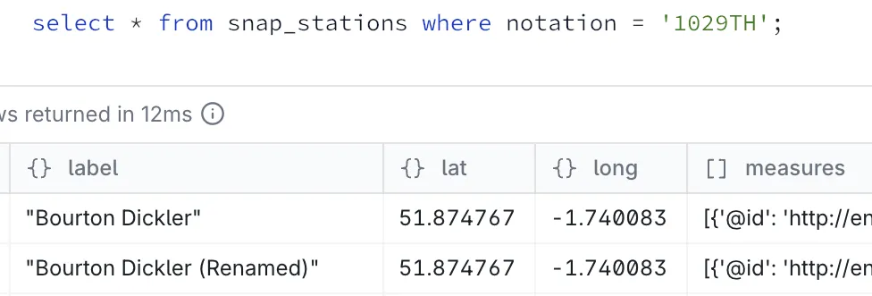
The devil is in the detail data 🔗
Sometimes data is just…mucky.
Here’s why we always use keys instead of labels—the latter can be imprecise and frequently changing:
SELECT notation, label, dbt_valid_from, dbt_valid_to
  FROM snap_stations
 WHERE notation = 'E6619'
 ORDER BY dbt_valid_to;
┌──────────┬──────────────────┬────────────────────────────┬────────────────────────────┐
│ notation │ label │ dbt_valid_from │ dbt_valid_to │
│ varchar │ json │ timestamp │ timestamp │
├──────────┼──────────────────┼────────────────────────────┼────────────────────────────┤
│ E6619 │ "Crowhurst GS" │ 2026-02-12 14:12:10.501256 │ 2026-02-13 20:45:44.391342 │
│ E6619 │ "CROWHURST WEIR" │ 2026-02-13 20:45:44.391342 │ 2026-02-13 21:15:48.618805 │
│ E6619 │ "Crowhurst GS" │ 2026-02-13 21:15:48.618805 │ 2026-02-14 00:46:35.044774 │
│ E6619 │ "CROWHURST WEIR" │ 2026-02-14 00:46:35.044774 │ 2026-02-14 01:01:34.296621 │
│ E6619 │ "Crowhurst GS" │ 2026-02-14 01:01:34.296621 │ 2026-02-14 03:15:46.92373 │
[etc etc]Eyeballing it, we can see this is nominally the same place (Crowhurst).
If we were using label as our join we’d lose the continuity of our data over time.
As it is, the label surfaced in a report will keep flip-flopping :)
Another example of upstream data being imperfect is this:
SELECT notation, label, measures[1].parameterName, dbt_valid_from, dbt_valid_to
  FROM snap_stations
 WHERE notation = '0'
 ORDER BY dbt_valid_to;
┌──────────┬───────────────────────────┬─────────────────────────────┬────────────────────────────┬────────────────────────────┐
│ notation │ label │ (measures[1]).parameterName │ dbt_valid_from │ dbt_valid_to │
│ varchar │ json │ varchar │ timestamp │ timestamp │
├──────────┼───────────────────────────┼─────────────────────────────┼────────────────────────────┼────────────────────────────┤
│ 0 │ "HELEBRIDGE" │ Water Level │ 2026-02-12 14:12:10.501256 │ 2026-02-13 17:59:01.543565 │
│ 0 │ "MEVAGISSEY FIRE STATION" │ Flow │ 2026-02-13 17:59:01.543565 │ 2026-02-13 18:46:55.201417 │
│ 0 │ "HELEBRIDGE" │ Water Level │ 2026-02-13 18:46:55.201417 │ 2026-02-14 06:31:08.75168 │
│ 0 │ "MEVAGISSEY FIRE STATION" │ Flow │ 2026-02-14 06:31:08.75168 │ 2026-02-14 07:31:14.07855 │
│ 0 │ "HELEBRIDGE" │ Water Level │ 2026-02-14 07:31:14.07855 │ 2026-02-14 16:16:23.465051 │
│ 0 │ "MEVAGISSEY FIRE STATION" │ Flow │ 2026-02-14 16:16:23.465051 │ 2026-02-14 16:31:45.420155 │
│ 0 │ "HELEBRIDGE" │ Water Level │ 2026-02-14 16:31:45.420155 │ 2026-02-15 06:31:07.812398 │Our unique key is notation, and there are apparently two measurements using it!
The same measures also have more correct-looking notation values, so one suspects this is an API glitch somewhere:
SELECT DISTINCT notation, label, measures[1].parameterName
  FROM snap_stations
 WHERE lcase(label) LIKE '%helebridge%'
    OR lcase(label) LIKE '%mevagissey%'
 ORDER BY 2, 3;
┌──────────┬───────────────────────────────────────┬─────────────────────────────┐
│ notation │ label │ (measures[1]).parameterName │
│ varchar │ json │ varchar │
├──────────┼───────────────────────────────────────┼─────────────────────────────┤
│ 0 │ "HELEBRIDGE" │ Flow │
│ 49168 │ "HELEBRIDGE" │ Flow │
│ 0 │ "HELEBRIDGE" │ Water Level │
│ 49111 │ "Helebridge" │ Water Level │
│ 18A10d │ "MEVAGISSEY FIRE STATION TO BE WITSD" │ Water Level │
│ 0 │ "MEVAGISSEY FIRE STATION" │ Flow │
│ 48191 │ "Mevagissey" │ Water Level │
└──────────┴───────────────────────────────────────┴─────────────────────────────┘Whilst there might be upstream data issues, sometimes there are self-inflicted mistakes. Here’s one that I realised when I started digging into the data:
SELECT s.notation, s.label,
       array_length(s.measures) AS measure_count,
       string_agg(DISTINCT m.parameterName, ', ' ORDER BY m.parameterName) AS parameter_names,
       s.dbt_valid_from, s.dbt_valid_to
  FROM snap_stations AS s
  CROSS JOIN UNNEST(s.measures) AS u(m)
 WHERE s.notation = '3275'
 GROUP BY s.notation, s.label, s.measures, s.dbt_valid_from, s.dbt_valid_to
 ORDER BY s.dbt_valid_to;
┌──────────┬────────────────────┬───────────────┬───────────────────────┬────────────────────────────┬────────────────────────────┐
│ notation │ label │ measure_count │ parameter_names │ dbt_valid_from │ dbt_valid_to │
│ varchar │ json │ int64 │ varchar │ timestamp │ timestamp │
├──────────┼────────────────────┼───────────────┼───────────────────────┼────────────────────────────┼────────────────────────────┤
│ 3275 │ "Rainfall station" │ 1 │ Rainfall │ 2026-02-12 14:12:10.501256 │ 2026-02-13 18:36:29.831889 │
│ 3275 │ "Rainfall station" │ 2 │ Rainfall, Temperature │ 2026-02-13 18:36:29.831889 │ 2026-02-13 18:46:55.201417 │
│ 3275 │ "Rainfall station" │ 1 │ Rainfall │ 2026-02-13 18:46:55.201417 │ 2026-02-13 19:31:15.74447 │
│ 3275 │ "Rainfall station" │ 2 │ Rainfall, Temperature │ 2026-02-13 19:31:15.74447 │ 2026-02-13 19:46:13.68915 │
│ 3275 │ "Rainfall station" │ 1 │ Rainfall │ 2026-02-13 19:46:13.68915 │ 2026-02-13 20:31:18.730487 │
│ 3275 │ "Rainfall station" │ 2 │ Rainfall, Temperature │ 2026-02-13 20:31:18.730487 │ 2026-02-13 20:45:44.391342 │
[…]Because we build the snapshot in dbt using a strategy of check and check_cols is all, any column changing triggers a new snapshot.
What’s happening here is as follows.
The station data includes measures, described in the API documentation as
The set of measurement types available from the station
However, sometimes the API is showing one measure, and sometimes two. Is that enough of a change that we want to track and incur this flip-flopping?
Arguably, the API’s return doesn’t match the documentation (what measures a station has available is not going to change multiple times per day?). But, we are the data engineers and our job is to provide a firebreak between whatever the source data provides, and something clean and consistent for the downstream consumers.
So, perhaps we should update our snapshot configuration to specify the actual columns we want to track. Which is indeed what dbt explicitly recommends that you do:
It is better to explicitly enumerate the columns that you want to check.
The tool that fits like a glove 🔗

The above section is a beautiful illustration of just how much sense the dbt approach makes. I’d already spent several hours analysing the source data before trying to build a pipeline. Even then, I missed some of the nuances described above.
With my clumsy self-built approach previously I would have lost a lot of the detail that makes it possible to dive into and troubleshoot the data like I just did. Crucially, dbt is strongly opinionated but ergonomically designed to help you implement a pipeline built around those opinions. By splitting out sources from staging from dimension snapshots from marts it makes it very easy to not only build the right thing, but diagnose it when it goes wrong. Sometimes it goes wrong from PEBKAC when building it, but in my experience a lot of the issues with pipelines come from upstream data issues (usually that are met with a puzzled "but it shouldn’t be sending that" reaction, or "oh yeah, it does that didn’t we mention it?").
Date dimension 🔗
Whilst the data about measuring stations and measurements comes from the API, it’s always useful to have a dimension table that provides date information. Typically you want to be able to do things like analysis by date periods (year, month, etc) which may or may not be based on the standard calendar. Or you want to look at days of the week, or any other date-based things you can think of.
Even if your end users are themselves writing SQL, and you’ve not got a different calendar (e.g. financial year, etc), a date dimension table is useful. It saves time for the user in remembering syntax, and avoids any ambiguities on things like day of the week number (is Monday the first, or second day of the week?). More importantly though, it ensures that analytical end users building through some kind of tool (such as Superset, etc) are going to be generating the exact same queries as everyone else, and thus getting the same answers.
There were a couple of options that I looked at. The first is DuckDB-specific and uses a FROM RANGE() clause to generate all the rows:
SELECT CAST(range AS DATE) AS date_day,
        monthname(range) AS date_monthname,
        CAST(CASE WHEN dayofweek(range) IN (0,6) THEN 1 ELSE 0 END AS BOOLEAN) AS date_is_weekend,
        […]
FROM range(DATE '2020-01-01',
            DATE '2031-01-01',
            INTERVAL '1 day')
The second was a good opportunity to explore dbt packages.
The dbt_utils includes a bunch of useful utilities including one for generating dates.
The advantage of this is that it’s database-agnostic; I could port my pipeline to run on Postgres or BigQuery or anything else without needing to worry about whether the DuckDB range function that I used above is available in them.
Packages are added to packages.yml:
packages:
  - package: dbt-labs/dbt_utils
    version: ">=1.0.0"
The date dimension table then looks similar to the first, except the FROM clause is different:
SELECT CAST(date_day AS DATE) AS date_day,
    monthname(date_day) AS date_monthname,
    CAST(CASE WHEN dayofweek(date_day) IN (0,6) THEN 1 ELSE 0 END AS BOOLEAN) AS date_is_weekend,
    […]
FROM (
        {{ dbt_utils.date_spine(
            datepart="day",
            start_date="cast('2020-01-01' as date)",
            end_date="cast('2031-01-01' as date)"
        ) }}
    ) AS date_spine
The resulting tables are identical; just different ways to build them.
SELECT * FROM dim_date LIMIT 1;┌────────────┬───────────┬────────────┬────────────────┬─────────────────┬────────────────┬─────────────────┬──────────────┬────────────────┬─────────────────┬──────────────┐
│ date_day │ date_year │ date_month │ date_monthname │ date_dayofmonth │ date_dayofweek │ date_is_weekend │ date_dayname │ date_dayofyear │ date_weekofyear │ date_quarter │
│ date │ int64 │ int64 │ varchar │ int64 │ int64 │ boolean │ varchar │ int64 │ int64 │ int64 │
├────────────┼───────────┼────────────┼────────────────┼─────────────────┼────────────────┼─────────────────┼──────────────┼────────────────┼─────────────────┼──────────────┤
│ 2020-01-01 │ 2020 │ 1 │ January │ 1 │ 3 │ false │ Wednesday │ 1 │ 1 │ 1 │
└────────────┴───────────┴────────────┴────────────────┴─────────────────┴────────────────┴─────────────────┴──────────────┴────────────────┴─────────────────┴──────────────┘SELECT * FROM dim_date_v2 LIMIT 1;┌────────────┬───────────┬────────────┬────────────────┬─────────────────┬────────────────┬─────────────────┬──────────────┬────────────────┬─────────────────┬──────────────┐
│ date_day │ date_year │ date_month │ date_monthname │ date_dayofmonth │ date_dayofweek │ date_is_weekend │ date_dayname │ date_dayofyear │ date_weekofyear │ date_quarter │
│ date │ int64 │ int64 │ varchar │ int64 │ int64 │ boolean │ varchar │ int64 │ int64 │ int64 │
├────────────┼───────────┼────────────┼────────────────┼─────────────────┼────────────────┼─────────────────┼──────────────┼────────────────┼─────────────────┼──────────────┤
│ 2020-01-01 │ 2020 │ 1 │ January │ 1 │ 3 │ false │ Wednesday │ 1 │ 1 │ 1 │
└────────────┴───────────┴────────────┴────────────────┴─────────────────┴────────────────┴─────────────────┴──────────────┴────────────────┴─────────────────┴──────────────┘Duplication is ok, lean in 🔗
One of the aspects of the dbt way of doing things that I instinctively recoiled from at first was the amount of data duplication. The source data is duplicated into staging; staging is duplicated into the marts. There are two aspects to bear in mind here:
-
Each layer serves a specific purpose. Being able to isolate, debug, and re-run as needed elements of the pipeline is important. Avoiding one big transformation from source-to-mart makes sure that transformation logic sits in the right place
-
There’s not necessarily as much duplication as you’d think. For example, the source layer is rebuilt at every run so only holds the current slice of data.
In addition to this…storage is cheap. It’s a small price to pay for building a flexible yet resilient data pipeline. Over-optimising is not going to be your friend here. We’re building analytics, not trying to scrape every bit of storage out of a 76KB computer being sent to the moon.
We’re going to do this thing properly: Tests and Checks and Contracts and more 🔗
This is where we really get into the guts of how dbt lies at the heart of making data engineering a more rigorous discipline in the way its software engineering older brother discovered a decade beforehand.
Any fool can throw together some SQL to CREATE TABLE AS SELECT a one-big-table (OBT) or even a star-schema.
In fact, I did just that!
But like we saw above with SCD and snapshots, there’s a lot more to a successful and resilient pipeline.
Making sure that the tables we’re building are actually correct, and proving so in a repeatable and automated manner, is crucial.
Of course, "correct" is up to you, the data engineer, to define. dbt gives us a litany of tools with which to encode and enforce it.
There are some features that are about the validity of the pipeline that we’ve built (does this transformation correctly result in the expected output), and others that validate the data that’s passing through it.
The configuration for all of these is done in the YAML that accompanies the SQL in the dbt project.
The YAML can be in a single schema.yml, or broken up into individual YAML files.
I quickly found the latter to be preferable for both source control footprint as well as simply locating the code that I wanted to work with.
Checking the data 🔗
Constraints provide a way to encode our beliefs as to the shape and behaviour of the data into the pipeline, and to cause it to flag any violation of these. For example:
-
Are keys unique? (hopefully)
-
Are keys NULL? (hopefully not)
Here’s what it looks like on dim_stations:
models:
  - name: dim_stations
    config:
      contract:
        enforced: true
    columns:
      - name: notation
        data_type: varchar
        constraints:
          - type: not_null
          - type: primary_key
You’ll notice the contract stanza in there.
Constraints are part of the broader contracts functionality in dbt.
Contracts also include further encoding of the data model by requiring the specification of a name and data type for every column in a model.
SELECT * might be fast and fun, but it’s also dirty af in the long run for building a pipeline that is stable and self-documenting (of which see below).
Data tests are similar to constraints, but whilst constraints are usually defined and enforced on the target database (although this varies on the actual database), tests are run by dbt as queries against the loaded data, separately from the actual build process (instead by the dbt test command).
Tests can also be more flexible and include custom SQL to test whatever conditions you want to.
Here’s a nice example of where a test is a better choice than a constraint:
models:
  - name: dim_measures
    columns:
      - name: notation
        tests:
          - not_null (1)
          - unique (1)
      - name: station
        tests:
          - not_null (2)
          - relationships:
              arguments: (3)
                to: ref('dim_stations') (3)
                field: notation (3)
              config:
                severity: warn (4)
                error_after: (4)
percent: 5 (4)| 1 | Check that the notation key is not NULL, and is unique |
| 2 | Check that the station foreign key is not NULL |
| 3 | Check that the station FK has a match… |
| 4 | …but only throw an error if this is the case with more than five percent of rows |
We looked at freshness of source data above.
This lets us signal to the operator if data has gone stale (the period beyond which data is determined as stale being up to us).
Another angle to this is that we might have fresh data from the source (i.e. the API is still providing data) but the data being provided has gone stale (e.g. it’s just feeding us readings data from a few days ago).
For this we can actually build a table (station_freshness):
SELECT notation, freshness_status, last_reading_at, time_since_last_reading, "label"
  FROM station_freshness;
┌──────────┬──────────────────┬──────────────────────────┬─────────────────────────┬──────────────────────────────────────────────┐
│ notation │ freshness_status │ last_reading_at │ time_since_last_reading │ label │
│ varchar │ varchar │ timestamp with time zone │ interval │ varchar │
├──────────┼──────────────────┼──────────────────────────┼─────────────────────────┼──────────────────────────────────────────────┤
│ 49118 │ stale (<24hr) │ 2026-02-18 06:00:00+00 │ 05:17:05.23269 │ "Polperro" │
│ 2758TH │ stale (<24hr) │ 2026-02-18 08:00:00+00 │ 03:17:05.23269 │ "Jubilee River at Pococks Lane" │
│ 712415 │ fresh (<1hr) │ 2026-02-18 10:45:00+00 │ 00:32:05.23269 │ "Thompson Park" │
│ 740102 │ fresh (<1hr) │ 2026-02-18 10:45:00+00 │ 00:32:05.23269 │ "Duddon Hall" │
│ E12493 │ fresh (<1hr) │ 2026-02-18 10:45:00+00 │ 00:32:05.23269 │ "St Bedes" │
│ E8266 │ fresh (<1hr) │ 2026-02-18 10:30:00+00 │ 00:47:05.23269 │ "Ardingly" │
│ E14550 │ fresh (<1hr) │ 2026-02-18 10:30:00+00 │ 00:47:05.23269 │ "Hartford" │
│ E84109 │ stale (<24hr) │ 2026-02-18 10:00:00+00 │ 01:17:05.23269 │ "Lympstone Longbrook Lane" │
│ F1703 │ dead (>24hr) │ 2025-04-23 10:15:00+01 │ 301 days 01:02:05.23269 │ "Fleet Weir" │
│ 067027 │ dead (>24hr) │ 2025-03-11 13:00:00+00 │ 343 days 22:17:05.23269 │ "Iron Bridge" │
│ 46108 │ dead (>24hr) │ 2025-05-28 10:00:00+01 │ 266 days 01:17:05.23269 │ "Rainfall station" │
[…]and then define a test on that table:
models:
  - name: station_freshness
    tests:
      - max_pct_failing: (1)
          config:
            severity: warn
          arguments:
            column: freshness_status (2)
            failing_value: "dead (>24hr)" (2)
threshold_pct: 10 (2)| 1 | This is a custom macro |
| 2 | Arguments to pass to the macro |
So dbt builds the model, and then runs the test.
It may strike you as excessive to have both a model (station_freshness) and macro (max_pct_failing).
However, it makes a lot of sense because we’re building a model which can then be referred to when investigating test failures.
If we shoved all this SQL into the test macro we’d not materialise the information.
We’d also not be able to re-use the macro for other tables with similar test requirements.
When the test runs as part of the build, if there are too many stations that haven’t sent new data in over a day we’ll see a warning in the run logs. We can also run the test in isolation and capture the row returned from the macro (which triggers the warning we see in the log):
❯ dbt test --select station_freshness --store-failures
[…]
14:10:53  Warning in test max_pct_failing_station_freshness_freshness_status__dead_24hr___5 (models/marts/station_freshness.yml)
14:10:53  Got 1 result, configured to warn if != 0
14:10:53
14:10:53    compiled code at target/compiled/env_agency/models/marts/station_freshness.yml/max_pct_failing_station_freshn_113478f1da33b78c269ac56f22cbec9d.sql
14:10:53
14:10:53    See test failures:
  -----------------------------------------------------------------------------------------------------------------------
  select * from "env-agency-dev"."main_dbt_test__audit"."max_pct_failing_station_freshn_113478f1da33b78c269ac56f22cbec9d"
  -----------------------------------------------------------------------------------------------------------------------
14:10:53
14:10:53  Done. PASS=1 WARN=1 ERROR=0 SKIP=0 NO-OP=0 TOTAL=2
SELECT * FROM "env-agency-dev"."main_dbt_test__audit"."max_pct_failing_station_freshn_113478f1da33b78c269ac56f22cbec9d";┌───────┬─────────┬─────────────┬───────────────┬────────────────────────────────────────┐
│ total │ failing │ failing_pct │ threshold_pct │ failure_reason │
│ int64 │ int64 │ double │ int32 │ varchar │
├───────┼─────────┼─────────────┼───────────────┼────────────────────────────────────────┤
│ 5458 │ 546 │ 10.0 │ 5 │ Failing pct 10.0% exceeds threshold 5% │
└───────┴─────────┴─────────────┴───────────────┴────────────────────────────────────────┘Checking the pipeline 🔗
Even data engineers make mistakes sometimes. Unit tests are a great way to encode what each part of a pipeline is supposed to do. This is then very useful for identifying logical errors that you make in the pipeline’s SQL, or changes made to it in the future.
Here’s a unit test defined to make sure that the readings fact table correctly unions data from the API with that from backfill:
unit_tests:
  - name: test_fct_readings_union (1)
    model: fct_readings (2)
    overrides:
      macros:
        is_incremental: false (3)
    given:
      - input: ref('stg_readings') (4)
        rows: (4)
          - { dateTime: "2025-01-01 00:00:00", measure: "api-reading", value: 3.5, } (4)
      - input: ref('stg_readings_archive') (5)
        rows: (5)
          - { dateTime: "2025-01-01 01:00:00", measure: "archive-reading", value: 7.2, } (5)
    expect: (6)
      rows: (6)
        - { dateTime: "2025-01-01 00:00:00", measure: "api-reading", value: 3.5, } (6)
- { dateTime: "2025-01-01 01:00:00", measure: "archive-reading", value: 7.2, } (6)| 1 | Name of the test |
| 2 | The model with which it’s associated |
| 3 | Since the model has incremental loading logic, we need to indicate that this unit test is simulating a full (non-incremental) load |
| 4 | Mock source row of data from the API (stg_readings) |
| 5 | Mock source row of data from the backfill (stg_readings_archive) |
| 6 | Expected rows of data |
If you want them to RTFM, you gotta write the FM 🔗
This is getting boring now, isn’t it. No, not this article. But my constant praise for dbt. If you were to describe an ideal data pipeline you’d hit the obvious points—clean data, sensible granularity, efficient table design. Quickly to follow would be things like testing, composability, suitability for source control, and so on. Eventually you’d get to documentation. And dbt nails all of this.
You see, the pipeline that we’re building is self-documenting. All the YAML I’ve been citing so far has been trimmed to illustrate the point being made alone. In reality though, the YAML for the models looks like this:
models:
  - name: dim_stations
    description: >
      Dimension table of monitoring stations across England. Each station has one or
      more measures. Full rebuild each run.
      🔗 [API docs](https://environment.data.gov.uk/flood-monitoring/doc/reference#stations)
    columns:
      - name: dateOpened
        description: >
          API sometimes returns multiple dates as a JSON array; we take
          the first value.
      - name: latitude
        description: Renamed from 'lat' in source API.
        […]
Every model, and every column, can have metadata associated with it in the description field.
The description field supports Markdown too, so you can embed links and formatting in it, over multiple lines if you want.
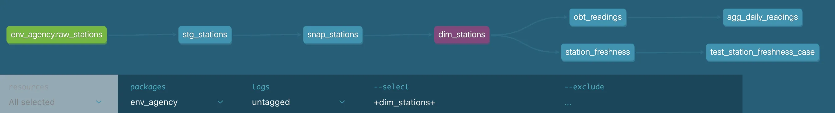
dbt also understands the lineage of all of the models (because when you create them, you use the ref function thus defining dependencies).
All of this means that you build your project and drop in bits of description as you do so, then run:
dbt docs generate && dbt docs serveThis generates the docs and then runs a web server locally, giving this kind of interface to inspect the table metadata:
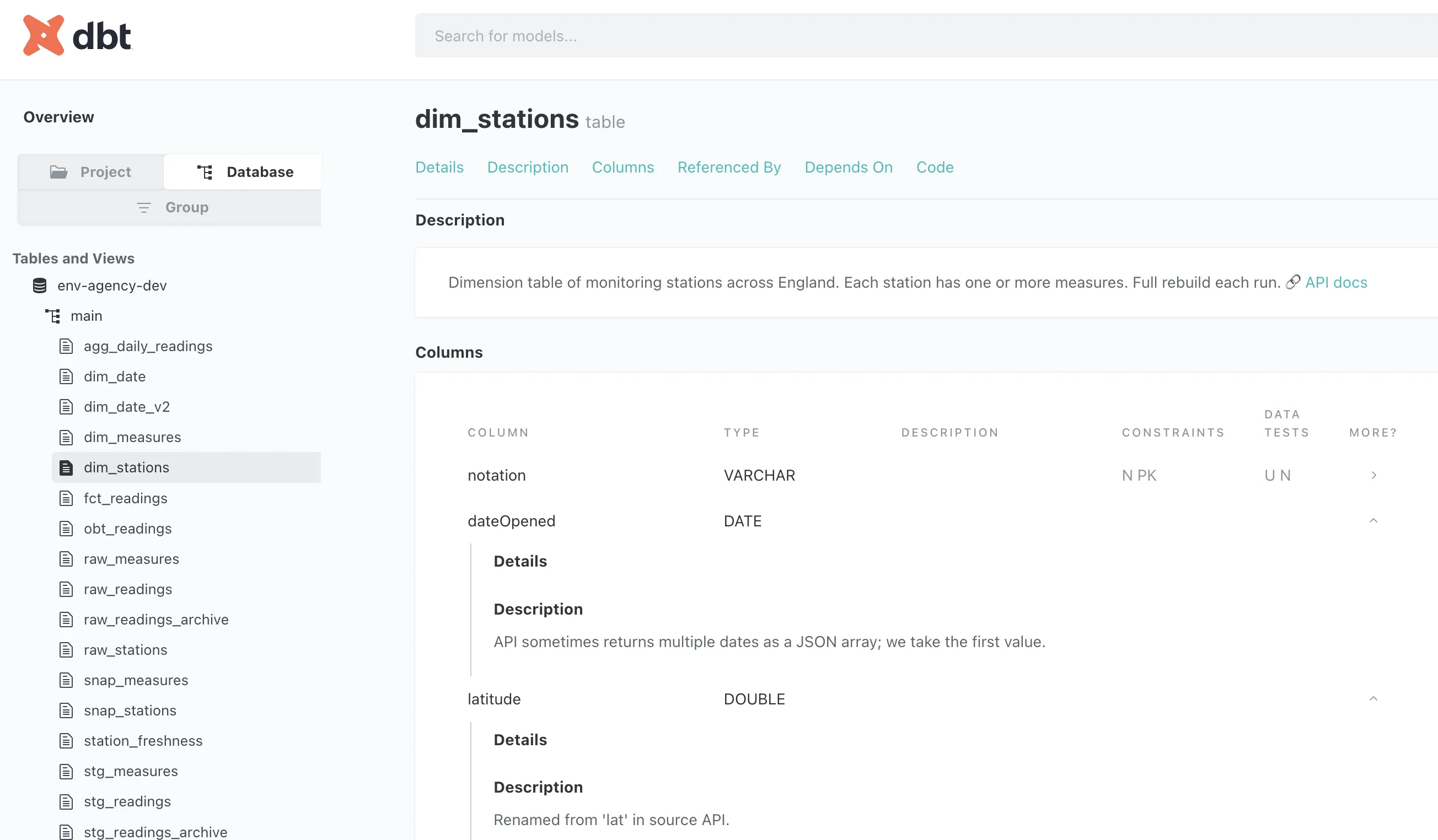
and its lineage:
Since the docs are built as a set of static HTML pages they can be deployed on a server for access by your end users. No more "so where does this data come from then?" or "how is this column derived?" calls. Well, maybe some. But fewer.
|
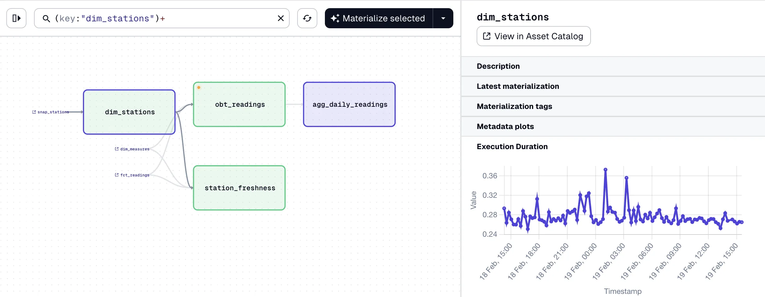
As a bonus, the same metadata is available in Dagster:
|
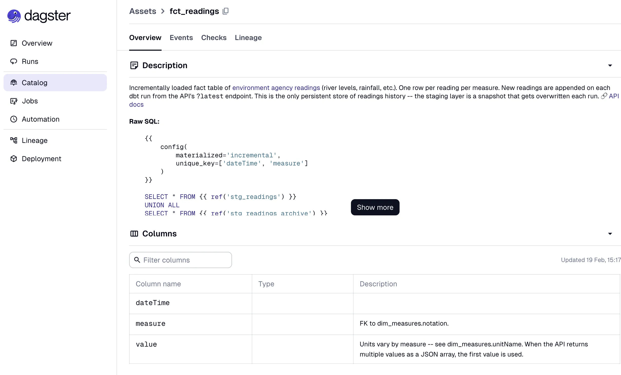
So speaking of Dagster, let’s conclude this article by looking at how we run this dbt pipeline that we’ve built.
Orchestration 🔗
dbt does one thing—and one thing only—very well. It builds kick-ass transformation pipelines.
We discussed briefly above the slight overstepping by using dbt and DuckDB to pull the API data into the source tables. In reality that should probably be another application doing the extraction, such as dlt, Airbyte, etc.
When it comes to putting our pipeline live and having it run automagically, we also need to look outside of dbt for this.
We could use cron, like absolute savages. It’d run on a schedule, but with absolutely nothing else to help an operator or data engineer monitor and troubleshoot.
I used Dagster, which integrates with dbt nicely (see the point above about how it automagically pulls in documentation). It understands the models and dependencies, and orchestrates everything nicely. It tracks executions and shows you runtimes.
Dagster is configured using Python code, which I had Claude write for me. If I weren’t using dbt to load the sources it’d have been even more straightforward, but to get visibility of them in the lineage graph it needed a little bit extra. It also needed configuring to not run them in parallel, since DuckDB is a single-user database.
I’m sure there’s a ton of functionality in Dagster that I’ve yet to explore, but it’s definitely ticking a lot of the boxes that I’d be looking for in such a tool: ease of use, clarity of interface, functionality, etc.
Better late than never, right? 🔗
All y’all out there sighing and rolling your eyes…yes yes. I know I’m not telling you anything new. You’ve all known for years that dbt is the way to build the transformations for data pipelines these days.
But hey, I’m catching up alright, and I’m loving the journey. This thing is good, and it gives me the warm fuzzy feeling that only a good piece of technology designed really well for a particular task can do.